Converting MBQC pattern to qiskit circuit and simulating it with Aer

In this example, we will demonstrate how to convert MBQC pattern to qiskit circuit and simulate it with Aer. We use the 3-qubit QFT as an example.

First, let us import relevant modules and define additional gates and function we’ll use:

import numpy as np
import matplotlib.pyplot as plt
import networkx as nx
import random
from graphix import Circuit
from graphix_ibmq.runner import IBMQBackend
from qiskit.tools.visualization import plot_histogram
from qiskit_aer.noise import NoiseModel, depolarizing_error


def cp(circuit, theta, control, target):
    """Controlled phase gate, decomposed"""
    circuit.rz(control, theta / 2)
    circuit.rz(target, theta / 2)
    circuit.cnot(control, target)
    circuit.rz(target, -1 * theta / 2)
    circuit.cnot(control, target)


def swap(circuit, a, b):
    """swap gate, decomposed"""
    circuit.cnot(a, b)
    circuit.cnot(b, a)
    circuit.cnot(a, b)

Now let us define a circuit to apply QFT to three-qubit state and transpile into MBQC measurement pattern using graphix.

circuit = Circuit(3)
for i in range(3):
    circuit.h(i)

psi = {}
random.seed(100)
# prepare random state for each input qubit
for i in range(3):
    theta = random.uniform(0, np.pi)
    phi = random.uniform(0, 2 * np.pi)
    circuit.ry(i, theta)
    circuit.rz(i, phi)
    psi[i] = [np.cos(theta / 2), np.sin(theta / 2) * np.exp(1j * phi)]

# 8 dimension input statevector
input_state = [0] * 8
for i in range(8):
    i_str = f"{i:03b}"
    input_state[i] = psi[0][int(i_str[0])] * psi[1][int(i_str[1])] * psi[2][int(i_str[2])]

# QFT
circuit.h(0)
cp(circuit, np.pi / 2, 1, 0)
cp(circuit, np.pi / 4, 2, 0)
circuit.h(1)
cp(circuit, np.pi / 2, 2, 1)
circuit.h(2)
swap(circuit, 0, 2)

# transpile and plot the graph
pattern = circuit.transpile()
nodes, edges = pattern.get_graph()
g = nx.Graph()
g.add_nodes_from(nodes)
g.add_edges_from(edges)
np.random.seed(100)
nx.draw(g)
plt.show()

Now let us convert the pattern to qiskit circuit.

# minimize the space to save memory during aer simulation
# see https://graphix.readthedocs.io/en/latest/tutorial.html#minimizing-space-of-a-pattern
pattern.minimize_space()

# convert to qiskit circuit
backend = IBMQBackend(pattern)
backend.to_qiskit()
print(type(backend.circ))

<class 'qiskit.circuit.quantumcircuit.QuantumCircuit'>

We can now simulate the circuit with Aer.

# run and get counts
result = backend.simulate()

We can also simulate the circuit with noise model

# create an empty noise model
noise_model = NoiseModel()
# add depolarizing error to all single qubit u1, u2, u3 gates
error = depolarizing_error(0.01, 1)
noise_model.add_all_qubit_quantum_error(error, ["u1", "u2", "u3"])

# print noise model info
print(noise_model)

NoiseModel:
  Basis gates: ['cx', 'id', 'rz', 'sx', 'u1', 'u2', 'u3']
  Instructions with noise: ['u1', 'u2', 'u3']
  All-qubits errors: ['u1', 'u2', 'u3']

Now we can run the simulation with noise model

# run and get counts
result_noise = backend.simulate(noise_model=noise_model)

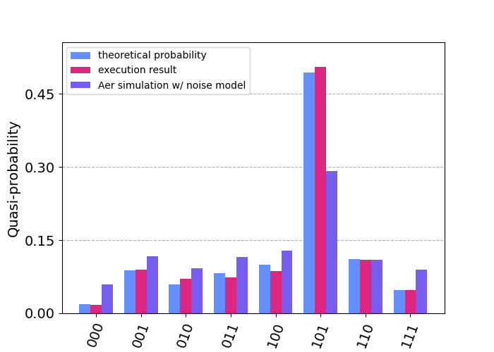
Now let us compare the results

# calculate the analytical
state = [0] * 8
omega = np.exp(1j * np.pi / 4)

for i in range(8):
    for j in range(8):
        state[i] += input_state[j] * omega ** (i * j) / 2**1.5

# rescale the analytical amplitudes to compare with sampling results
count_theory = {}
for i in range(2**3):
    count_theory[f"{i:03b}"] = 1024 * np.abs(state[i]) ** 2

# plot and compare the results
fig, ax = plt.subplots(figsize=(7,5))
plot_histogram([count_theory, result, result_noise],
               legend=["theoretical probability", "execution result", "Aer simulation w/ noise model"],
               ax=ax,
               bar_labels=False)
legend = ax.legend(fontsize=18)
legend = ax.legend(loc='upper left')